
Easily group columns in excel tables with LOTS of columns, hide them clearly and aesthetically using a slicer

If you have many columns in your Excel file, it can sometimes be quite difficult to find the information you are looking for.
It's a good idea to group columns and ungroup them as needed. but k Excel's built-in grouping function is frankly terribly difficult and useless.
In this article you will find how to use slicers to group and hide columns in excel table.

Table In this example, it is a customer table. We have additional columns about the project, sales and interview notes.
This will help you navigate easily.
No VBA coding knowledge is required with this solution. You just need to copy and paste the code.
To explain step by step;
1) create 4 empty rows over your table. We will enter parameters related to filtering. Also, the slicer will be located here.

We have two pages in the file. The first is the page with the data. the other is the grouping items page.
2) Write the Grouping Items on the Items page.
Add a sequence number to the beginning of the group items. This will help us sort the slicer easily. In the second column, write the ID numbers respectively.
3) turn your list into a table.
Select the table and press the insert table button. Click OK.
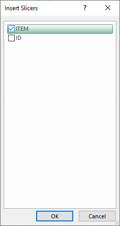
4) Add slicer
Add slicer from the "Table properties" tab, click "items" in the list that will open. check that it is working.
5) Add a cell that calculates something
Click anywhere other than the table. Click autosum and select the Identity column. This will trigger our "calculate" code.

6) Cut the slicer from here and paste it on our homepage.
It is more accurate to set the slicer horizontally. Increase the number of columns from the Slicer tab.

7) In line 4, write the group number of each column.
If you want a column to appear in more than one group, type the two group numbers with a comma between them.
Type 0 in line 4 for the columns you want to appear continuously regardless of the group selection.

Set line 4 to text.
8) Copy and paste the code
Private Sub Worksheet_Calculate()
'this event triggered when the slicer items change.
Dim selectedmenu(10) As String
Dim showcolumn(100) As Boolean
Dim clx, rng As Range
'settings
mysheet = "MYSHEET"
myfilterrow = 4
'read group definition on items sheet
Q = 1
With Worksheets("items")
lastrow = WorksheetFunction.CountA(Range("B2:B20")) 'last row of the items
rngtxt = "B2:B" + LTrim$(Str$(lastrow)) 'set range of the item list
Set rng = Worksheets("items").Range(rngtxt) 'set the selected item range
'loop on group names filtered by the slicer
'and assign them into an array
For Each clx In rng.SpecialCells(xlCellTypeVisible)
If clx.Value = "" Then Exit For 'in case the table range shorten due to deletetion of the rows
d = clx.Row
If .Cells(d, 1) = "" Then Exit For
selectedmenu(Q) = LTrim$(Str$(.Cells(d, 2)))
Q = Q + 1
jump:
Next
End With
With Worksheets(mysheet)
columnx = 1
rowx = myfilterrow
Dim MyArray() As String
'loop on the columns, read the row nr4
'and compare with the array
For K = 1 To 100
For J = 1 To Q - 1
txt = (.Cells(myfilterrow, K))
MyArray() = Split(txt, ",")
If txt <> "" Then
For N = 0 To UBound(MyArray())
If MyArray(N) = selectedmenu(J) Or MyArray(N) = "0" Then
showcolumn(K) = True
End If
Next
End If
Next
Next
'hide or show each column by variable showcolumn()
For C = 1 To 100
.Columns(C).EntireColumn.Hidden = Not showcolumn(C)
Next
.Cells(5, 1).Select
End With
End Sub
Press Alt F11 in Excel Find the items row in the list on the left and double-click it.
Paste the code into the white space on the right.
Close the editor.
9 Test it.
columns are hidden and shown according to our slicer selection.
I hope that will be useful.
Comments